Qosmo
Neutone Blog
In this article, we’ll briefly go over how neural networks can be used as a new type of audio effect called timbre transfer. Timbre transfer is an audio effect that changes the timbre of the input audio into some certain style. We’ll cover two recent architectures in this field: DDSP and RAVE.
Also, we will look at how you can train your own RAVE models and use them with our VST plugin, neutone.
Autoencoders
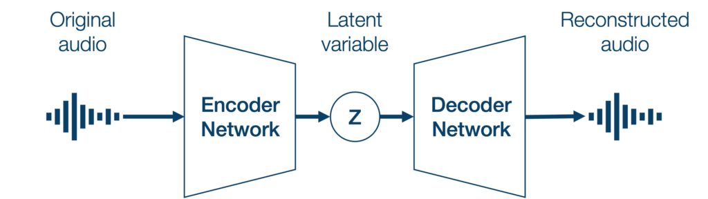
Autoencoders are neural networks that are trained to compress and then reconstruct the input. The network can be split into two parts: encoder and decoder. The encoder compresses (encodes) the data into an intermediate representation (often referred to as the latent variable). This intermediate representation may contain information about the musical performance such as pitch or loudness. From this intermediate representation, the decoder tries to reconstruct (decode) the original input.
At first glance, the autoencoder seems pointless, as it tries to reconstruct whatever input it is fed. However this can be used as a timbre transfer effect when you feed sounds that are different from what the training data. For example, an autoencoder that is trained on violin sounds can only reconstruct violin sounds. So, when it is fed flute sounds as input, it transfers the timbre into that of a violin.
DDSP
DDSP (Differentiable Digital Signal Processing) refers to the incorporation of traditional DSP techniques in a deep learning framework. The basic DDSP model proposed by Engel et al. is an autoencoder-like model architecture with a DDSP-based synthesizer to produce the final output. Basically, it is specialized for musical sounds where the frequencies present in a sound is a multiple of the fundamental frequency. For example, when you play a note on some instrument at A4 (440Hz), there are overtones present at 880Hz, 1320Hz and so on. First, the encoder estimates the loudness and the fundamental frequency of the sound. Then, the decoder estimates the amplitude of each overtone and the DDSP synthesizer synthesizes the final output audio from those estimated parameters. You can read more about DDSP here.
The advantages of DDSP is that the assumptions it makes on the harmonicity of the sound allows it to efficiently train with high quality. Also, since the synthesizer is strictly conditioned on the fundamental frequency, it tends to follow the pitch of the input better than models like RAVE. On the other hand, these assumptions limits the type of sounds it can model. For example, DDSP cannot model percussions with no harmonic structure and polyphonic instruments like pianos that do not have a single fundamental frequency.
DDSP models will be available for neutone in late July.
RAVE
RAVE (ReAltime Variational autoEncoder) is a VAE (Variational AutoEncoder) that encodes and decodes raw audio with convolutional neural networks (Caillon and Esling, 2022). RAVE employs many advanced techniques (such as PQMF sub-band coding) to make it fast enough to work in realtime in a CPU, whereas previous methods could not. It also utilizes a discriminator network similar to a GAN (Generative Adversarial Network) to improve the output quality.
As it processes raw audio without any assumptions, any type of sounds can be modeled by RAVE. The disadvantage compared to DDSP is that it is more computationally expensive to train (approximately 3 days on a RTX 3080), and requires more data to train (2~3 hours of training data or more).
Training RAVE models
As of 2022, there are two options for training RAVE models:
- Original training script for RAVE
- You need a decent NVIDIA GPU (with a VRAM > 6GB).
- You also need to install requirements like python, pytorch+CUDA, etc.
- Colab notebook for RAVE
- The free plan has limits for GPU usage.
- It would be very difficult to fully train a RAVE model without paying premium.
Preparing the training data
Preparing a good training data is the most difficult part of training RAVE models. While there are no sure-fire ways to prepare the perfect dataset, here are some tips:
- Data preprocessing maybe required for good results.
- Gain normalization is necessary if the original data is relatively quiet.
- A model trained on quiet sounds can behave erratically when it is fed loud sounds as input.
- Gain normalization is necessary if the original data is relatively quiet.
- Choosing a good data.
- Recording a long solo performance of a certain instrument is effective and often leads to clean results.
- For example, RAVE.drumkit was trained on a large dataset of many performances using a single drum kit.
- Recording environment should ideally be similar across the dataset.
- Some amount of variety in the data is good, but too much variety brings poor results.
- Training the model on exhaust note of a bike sitting idle for few hours resulted in a model that produces similar output no matter the input.
- Training the model on several thousand different drum sounds resulted in a model that produces muddy output that sounds like the mix of several drum sounds.
- Recording a long solo performance of a certain instrument is effective and often leads to clean results.
- Some trial and error is necessary for making good models……
- It’s hard to predict how the trained model will react to different input sounds.
Parameters for training RAVE
Training on Colab should be straight forward. Configure the training settings using the text fields and check boxes, and execute the cells up to the “train RAVE” part. The prior training can be ignored for timbre transfer purposes.
The training script can be run by following the directions given by running cli_helper.py, or as:
python train_rave.py --name [name] -c [small/large/default] --wav [directory of wav files] --preprocessed [some directory with fast read speed] --no-latency [true/false]
There are some arguments for both python script/Colab that should be looked at:
-
--name/training_name- The output directory.
-
--wav/input_dataset- Audio files will be searched for recursively from this directory.
-
--preprocessed(only for python script)- RAVE reads the files in the –wav directory and cuts them up into 1s sections, saving them into a database file.
- The database file is stored in the directory specified with this flag.
- Ideally, this should be somewhere with fast read speed, like an SSD.
- Check your GPU utility % with
nvidia-smi. If it is low, your disk speed maybe the bottleneck for the training speed.
- Check your GPU utility % with
-
--no_latency/no_latency_mode- Can be true (checked) or false (unchecked). Default value is false.
- With this flag set to
true, the model uses causal convolutions instead of standard convolution.- Normal convolution needs information about the future input which causes lookahead latency.
- Causal convolutions can run in realtime with little latency, but with slightly worse quality than standard convolution.
- When set to false, latency is approximately half a second with the default size model.
- Since this is very large for an audio effect we recommend setting this flag to
true - Also, large model takes much longer to train.
- Since this is very large for an audio effect we recommend setting this flag to
-
-c/size- Can be large, small or not specified at all (default).
- Controls the size of the model.
-
smallordefault(medium size) is recommended, since large model is CPU intensive.
-
-sr/sampling_rate- Default sample rate is 48000Hz/44100Hz(Colab)
- Current version of neutone only supports 48000Hz, so it is better to train with 48000 for now.
Exporting the model
Before wrapping the model for use in neutone, we have to export the model into torchscript format.
python export_rave.py --run [path to saved checkpoint file] --cached true --sr 48000
Make sure to set
--cached truefor realtime-compatible convolution (see next section for details).
Streaming Convolution for Realtime Audio Models
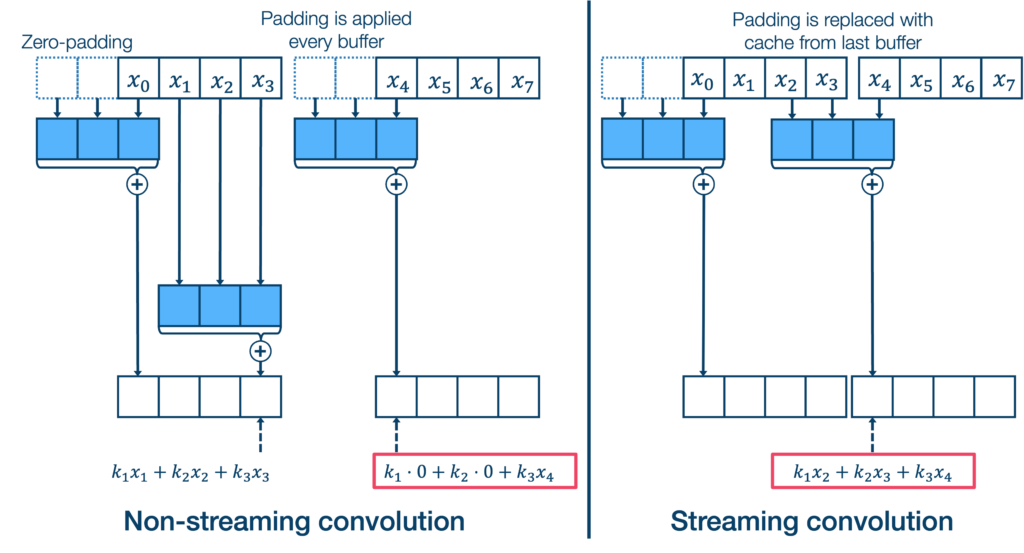
In a realtime audio effect, the model must process each buffer of audio one-by-one. But we want to process the audio in a way that is equivalent to processing the entire audio. For a model with convolutional layers, this becomes a problem. If we use standard convolution, unnecessary zero-padding will be added before (and after, in case of non-causal convolutions) every buffer, which messes up the continuity between buffers. Had we processed these buffers together with convolution, this zero-padding would not have been applied. Thus, a streaming convolution stores information from the previous buffer in a cache, which is used as the padding of the current buffer instead of zero-padding.
A simple implementation is shown in the example overdrive script of neutone_sdk. A more detailed explanation and a full implementation including Transposed Convolution will be added soon as well. In the meantime you can also check out the implementation used in RAVE and read this excellent article by Andrew Gibiansky, or this paper by the authors of RAVE.